How our tennis prediction algorithm works (hybrid AI + stats)

Algorithm hub — Part 1 of 3. This article explains how our hybrid tennis prediction pipeline is built, validated, and tracked in production. Continue with Part 2: prediction features and Part 3: ML vs statistical models. See also the technology overview and today's live predictions.
If you bet tennis—or you simply want to understand why one player is priced like a lock while another looks “cheap”—you need a prediction story that is honest about what “accuracy” means. This article explains how TennisPredictor turns structured match data into calibrated win probabilities, why bookmaker-implied probabilities sit at the top of our feature importance table, and how three different accuracy numbers (cross-validation, strict holdout test, and live settled picks) can all be true at once.
Headline claim (“70%+”): our rolling live accuracy on settled predictions has recently printed about 72% correct on a tracked sample (see the live results section). Season-wide reviews (for example our 2025 season recap) have reported similar ~71% hit rates when measured over larger verified batches. Those figures are not the same thing as the 63.1% holdout test score on the latest chronological slice—read on for why that gap is expected, not a contradiction.
How to read this article (if you only have two minutes)
If you care about betting: jump to Betting angle after skimming the model snapshot table—then read Live accuracy so you understand why a 127-match scored batch is informative but not “proof” in a statistical-testing sense.
If you care about machine learning: pay attention to the feature-importance section and the CV vs holdout chart. Those two pieces prevent the classic failure mode of quoting training-curve optimism as if it were deployment reality.
If you care about intellectual honesty: read Three “accuracy” definitions before tweeting a single percentage as “the model accuracy.” Tennis prediction has multiple legitimate definitions; mixing them is how bad takes get manufactured.
Why tennis match prediction is genuinely hard
Tennis is not basketball with substitutions. The same two players can produce wildly different outcomes week to week because:
- Surface changes the game — clay reward structures differ from indoor hard courts.
- Form is non-stationary — injuries, coaching changes, and confidence swings move faster than rankings.
- Small samples dominate perception — a hot month can be signal or noise.
- The market is informed — closing lines aggregate enormous information; beating them requires edge, not vibes.
Naive “pick the higher rank” rules often land in the mid‑50% to low‑60% band depending on era and sample—better than a coin flip, but not enough to survive margin and staking friction. Our job is to combine player history, market prices, and context features in a model that generalises to future matches.
There is also a uncomfortable truth that good modellers accept early: the market is often right. Closing lines reflect injuries, insiders, coaching changes, and millions of dollars of information aggregation. That is exactly why implied probability features rank so highly in our forest: they are not “cheating”—they are a compressed sensor of consensus. The model’s job is not to prove the market stupid every Tuesday; it is to find structured deviations where our features justify a different fair price.
What we ship today (high level)
The production pipeline you interact with on the dashboard is built around a supervised learning setup:
- Label: did player 1 win the match (yes/no)?
- Features: hundreds of numeric signals per match—rank gaps, surface-specific win rates, rest, market odds and implied probabilities, interactions, and more.
- Model: a Random Forest classifier (latest training snapshot: 9,829 labelled examples, 292 input features) with chronological validation so we do not “peek” at future results when measuring generalisation.
We still layer business rules on the product side (confidence bands, presentation, and quality checks). The machine-learning core is the workhorse that turns features into a win probability you can compare to the book.
Random Forests in one paragraph (no equations)
A Random Forest trains many decision trees on random subsets of rows and features, then averages their votes. Each tree asks a sequence of yes/no questions—“Is the rank gap above this threshold?”, “Is player 1’s clay win rate higher than player 2’s?”—until it reaches a leaf that outputs a probability directionally consistent with the training labels.
Why we like forests for tennis:
- They handle non-linear interactions without forcing you to hand-write every crossover term.
- They are relatively robust to scaling quirks when many features live on different numeric ranges.
- They produce importance scores that are easy to audit in plain language (even if some raw feature names are technical).
They are not a personality cult: forests can overfit if you leak future information, reward spurious correlations on tiny samples, or look amazing on CV while struggling on a truly forward holdout. That is why we pair them with chronological evaluation and live monitoring.
Production model snapshot (latest training metadata)
| Metric | Value |
|---|---|
| Algorithm | Random Forest (200 trees, max depth 15) |
| Training examples | 9,829 |
| Input features | 292 |
| 5-fold CV mean accuracy | 79.5% |
| CV standard deviation | 6.1% |
| Chronological holdout test accuracy | 63.1% |
The CV vs holdout spread is large—that is normal when the test window is harder or distributional shift creeps in (new players, schedule compression, market tightening). The charts later make this visually obvious.
Chronological splits: why “random test sets” are not enough
If you shuffle matches and hide 20% as a test set, you can accidentally allow future information to leak into past rows through players who appear many times across seasons. Tennis is a time series of human beings, not independent coin flips.
A chronological protocol instead says: train on an older era, score a newer era, the way you would actually deploy. That typically reduces headline accuracy versus a random split—but it increases trust. The 63.1% holdout figure is meaningful precisely because it refuses the comforting fiction of i.i.d. rows.
Feature importance: what the model actually leans on
We export permutation-style feature rankings from the trained Random Forest. The takeaway is blunt: market-derived inputs (decimal odds and implied probabilities) absorb a huge share of total importance, alongside rank gaps and win-rate differentials.
What this means for bettors:
- If our probability matches the implied odds, there may be no structural edge—you still need price.
- When our model and the market diverge materially, that is where value conversations start—always subject to stake limits and uncertainty.
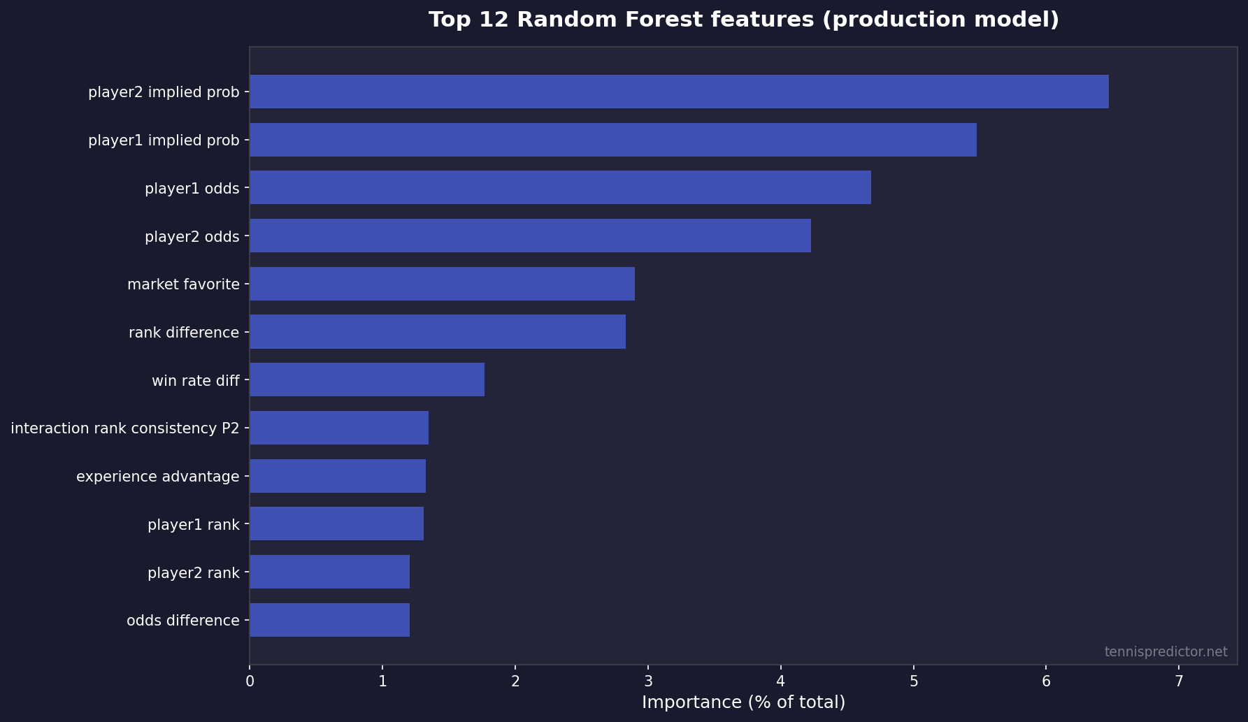
Figure 1: Top 12 features by importance share (sum of importances = 100% across all 292 features).
Top 10 features (exact shares)
| Rank | Feature (as logged in training) | Importance share |
|---|---|---|
| 1 | player2_implied_prob | 6.47% |
| 2 | player1_implied_prob | 5.48% |
| 3 | player1_odds | 4.68% |
| 4 | player2_odds | 4.23% |
| 5 | market_favorite | 2.90% |
| 6 | rank_difference | 2.83% |
| 7 | win_rate_diff | 1.77% |
| 8 | interaction_rank_consistency_p2 | 1.34% |
| 9 | experience_advantage | 1.32% |
| 10 | player1_rank | 1.31% |
For a plain-language tour of how we think about form, surface, and H2H—beyond raw column names—read The secret sauce: features that power our tennis predictions.
Why odds live inside the model (and why that is not “copying the line”)
Bettors sometimes hear “the model uses odds” and assume the system must be circular: “If you start from the price, you end at the price.” That misunderstands what supervised learning is doing.
Odds are not a label; they are inputs. The label remains who won. The model learns residual structure: where player-specific surface trends, fatigue, schedule density, or stylistic mismatches systematically push outcomes away from what a naive market-implied probability might suggest—when those signals are stable enough to generalise.
This is also why “beat the closing line” remains the professional standard for betting value: our probabilities are best treated as fair-win-rate hypotheses you must compare to prices you can actually bet, not as a moral victory over a screenshot of a model number.
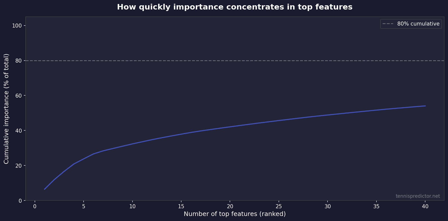
Figure 2: Cumulative importance by rank—most signal sits in a relatively small number of top features.
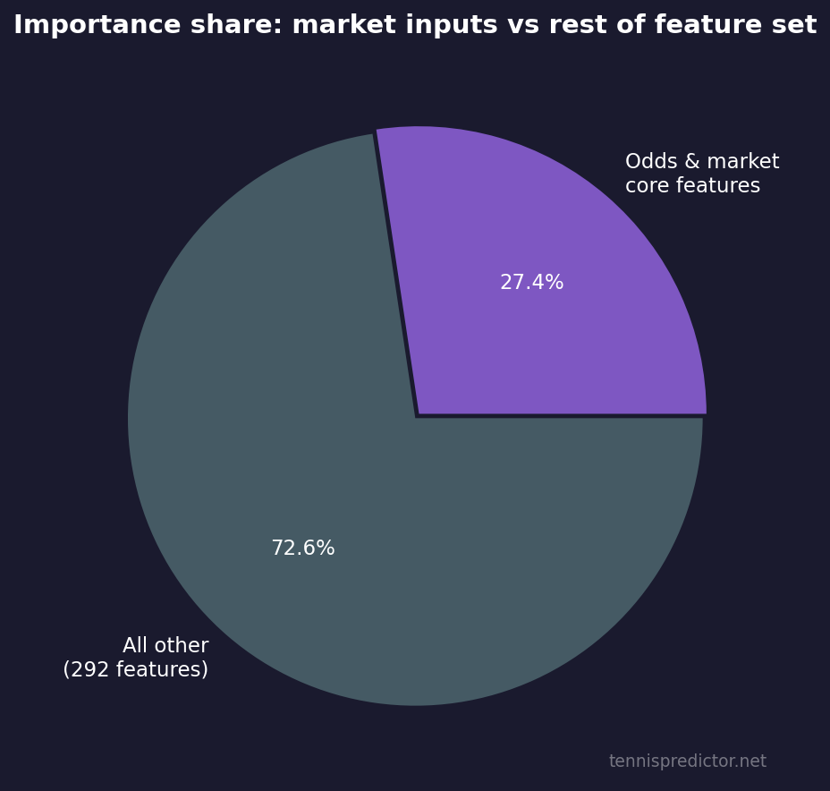
Figure 3: Approximate share of total importance captured by odds- and market-linked inputs vs everything else (292 features total).
Validation: cross-validation vs a strict holdout test
Academic honesty matters. Cross-validation answers: “How stable is training on different folds?” A chronological holdout answers: “If we pretend we only know the past, how well do we score the immediate future?”
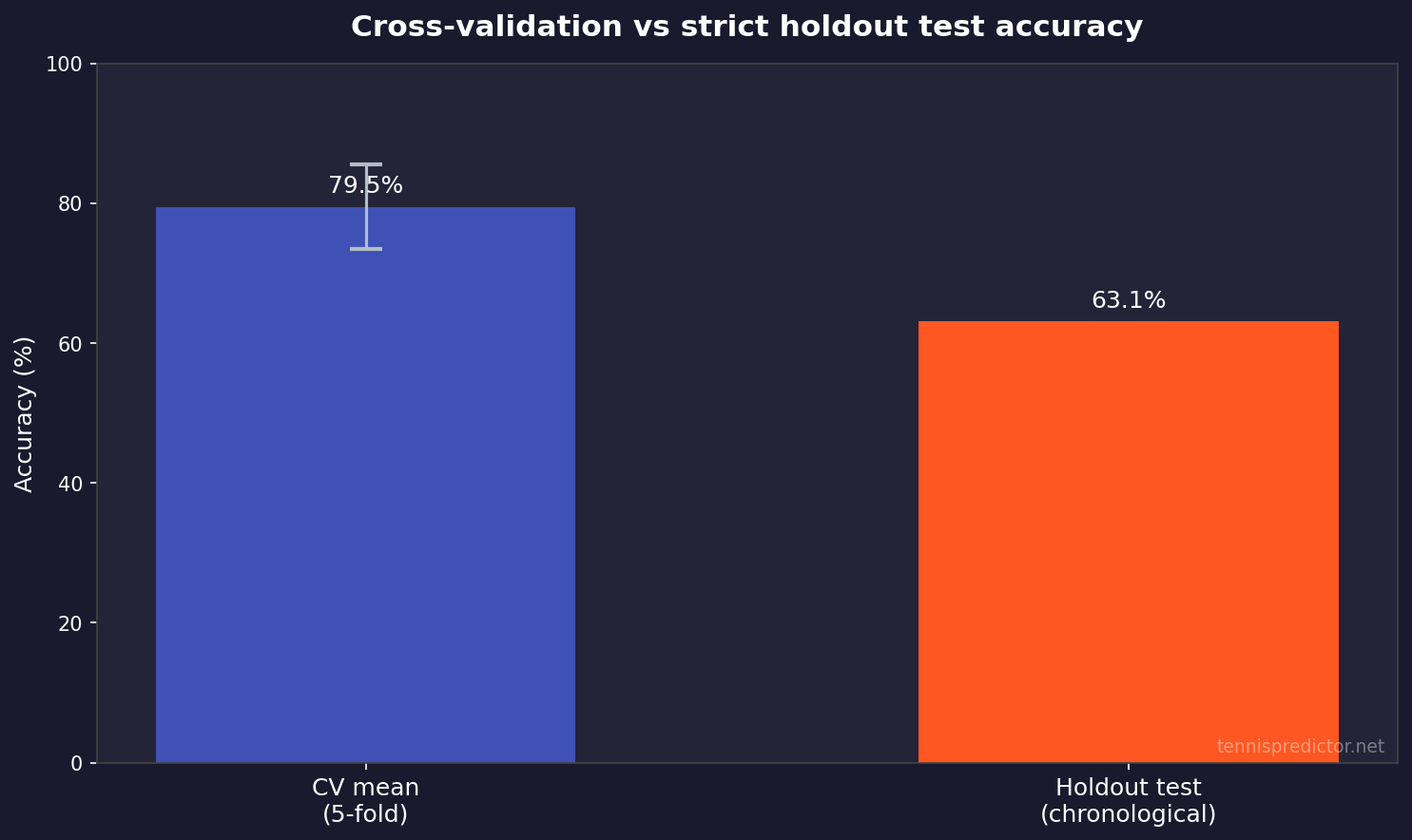
Figure 4: 5-fold CV mean (with ±1 SD error bar) vs holdout test accuracy on the latest metadata export.
How to read it:
- CV ~79.5% tells you the model is learnable and not hopelessly noisy on historical structure.
- Holdout ~63.1% tells you real forward generalisation on the held-out time window is more conservative—as it should be when conditions change.
If you only ever quoted CV, you would oversell. If you only ever quoted holdout, you might undersell live performance when the product filters for higher-confidence spots. That is why we publish multiple views.
A toy example: implied probability vs “fair” probability
Suppose a book lists 1.80 decimal odds for player A. Ignoring margin, the implied win chance is 1 ÷ 1.80 ≈ 55.6%. If our model outputs 58% for player A, the directional betting question is whether 58% is far enough above 55.6% to cover margin, variance, and execution—not whether “58% is high.”
If our model outputs 52% while the market implies 55.6%, the model is effectively saying the favourite is slightly overbet relative to our features—even if player A might still win half the time. Accuracy statistics will never replace that price-relative reasoning.
Live accuracy: settled predictions and confidence buckets
Offline metrics are not fan experience. We also track live predictions where outcomes have settled, and we bucket by confidence bands maintained inside our KPI tooling.
Latest snapshot (internal KPI file, updated 2026-04-17):
| KPI | Value |
|---|---|
| Predictions logged (total) | 1,556 |
| Settled / scored | 127 |
| Correct | 91 |
| Rolling accuracy (91 ÷ 127) | 71.65% |
Important caveats:
- The 127 scored matches are a small sample—confidence intervals are wide; use this as a health check, not a guarantee.
- Accuracy rises with confidence bucket in our tracking—exactly what you want if probabilities are remotely calibrated.
Sampling nuance: the “total predictions logged” count can be much larger than “settled” because many fixtures are future-facing, cancelled, or not yet reconciled in the KPI pipeline when the snapshot is taken. That is normal in live systems. The headline 71.65% is explicitly conditional on being in the scored set.
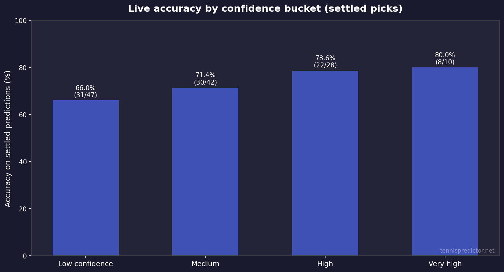
Figure 5: Settled accuracy by confidence bucket from the same KPI snapshot (counts shown on bars).
For a narrative tour across a full season—with tournament context—see The 2025 tennis season in review.
Three “accuracy” definitions side by side
| Measure | What it answers | Latest headline figure |
|---|---|---|
| 5-fold CV mean | Stability across training folds | 79.5% (± 6.1% SD) |
| Chronological holdout test | Strict forward generalisation on held-out matches | 63.1% |
| Live settled hit rate | What happened after deployment, when results are known | 71.65% (91/127 in KPI snapshot) |
None of these numbers replaces bankroll logic. They answer different questions.
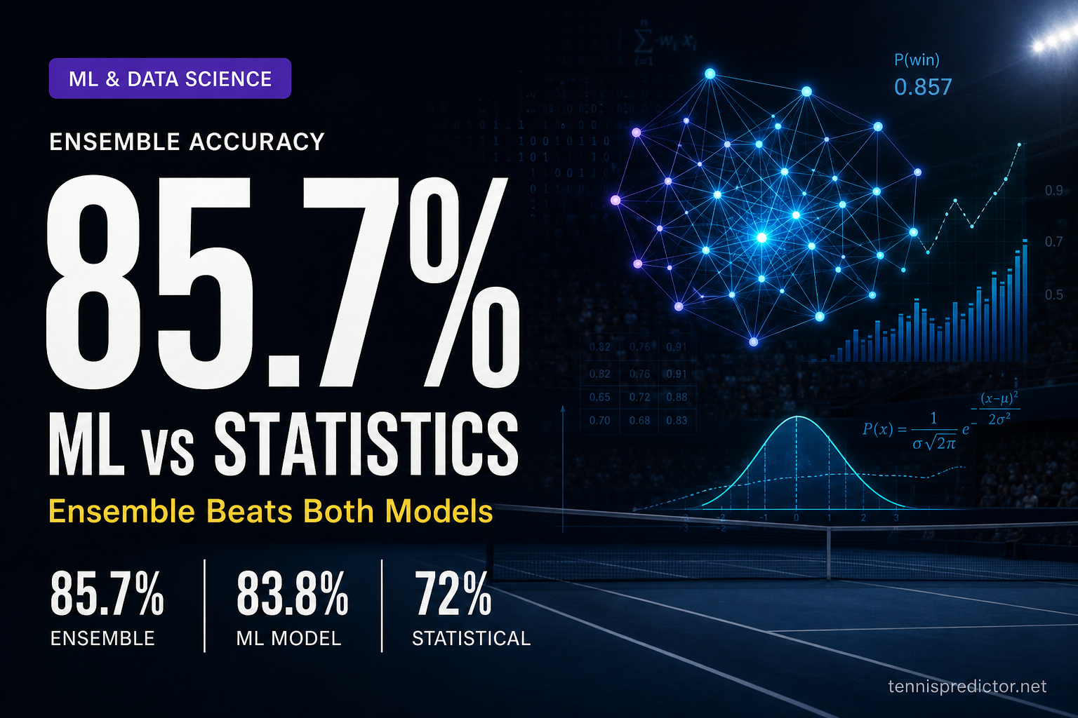
How we combine intuition from multiple model philosophies
We are not religious about a single algorithm in isolation—see the head-to-head write-up in Machine learning vs statistical models: which predicts tennis better?. In product terms:
- Tree-based learning captures non-linear interactions (rank gaps × surface × rest).
- Market features anchor probabilities to what the world already knows.
- Rule-based checks keep outputs usable when data is thin (early rounds, wildcards, first-time meetings).
That combination is why we still talk about an ensemble mindset even when a Random Forest is the heavy lifter in the current training export.
Betting angle: how to use the dashboard without fooling yourself
When you open the dashboard, treat probabilities as decision inputs, not lottery tickets.
Practical habits:
- Compare our win probability to implied probability from odds before staking.
- Prefer spots where model confidence and model–market agreement line up—disagreement is often where variance lives.
- Scale stakes to confidence and liquidity; ignore anyone promising flat “unit” outcomes across all price ranges.
- Track your own results separately; public accuracy stats will never map 1:1 to your closing lines.
Confidence bands: what they are (and are not)
A higher confidence band is supposed to mean “we think the signal is clearer,” not “free money.” Tennis still contains injury surprises, bad days, and plain randomness—especially in volatile matchups between two high-variance shotmakers.
Use confidence as a prioritisation tool: when time is limited, start with matches where:
- The probability is stable across similar historical contexts (surface, tournament tier, rest), and
- Your edge vs price still clears margin after you account for staking constraints.
Value hunting without cosplaying as a quant
You do not need a PhD to apply a disciplined filter:
- Write down our win probability.
- Convert odds to implied probability.
- Ask whether the gap survives margin (books are not fair coins).
- Only then ask whether your bankroll can survive the variance of that bet type.
If you want a deeper dive on mistakes that survive even “good” models, pair this article with our betting-strategy pieces linked from the blog index—bankroll discipline remains the great filter that accuracy percentages never replace.
What we do not claim
We do not claim:
- A magical fixed percentage that applies to every week of the season.
- That short-term live samples are statistically stable (they vary).
- That long-run profitability is automatic if headline accuracy exceeds 70%—price and staking dominate.
Coverage and fairness constraints
Tennis is global; data availability is not uniform across tours, challengers, and women’s events at the same granularity as flagship ATP stops. When sample sizes for a player are thin—returning from injury, first tournament on clay, wildcard chaos—uncertainty should rise. A model that does not widen uncertainty in those settings is a model lying to you in a soothing voice.
We also avoid presenting fabricated “case study” matches with scores and player names unless they are sourced and verified like a statistics paper. Betting content is full of memorable stories; we prefer reproducible aggregates you can audit.
Continuous improvement (where the roadmap actually shows up)
We iterate on the same levers most serious sports modelling teams use:
- Retrain as new completed matches arrive.
- Re-evaluate feature drift (young players, surface calendar shifts).
- Recalibrate probability bands when market structure changes.
- Expand coverage carefully—more tournaments only help if labels stay clean.
What “calibration” means in plain English
A model can be accurate in the narrow sense—often right on favourites—while still being miscalibrated in the probabilistic sense: it might say “70%” in situations that only convert 62% of the time. Calibration work tries to align stated probabilities with long-run frequencies within comparable buckets.
That is one reason we track confidence buckets on live settled picks. If “80%” statements only win 62% of the time, something is wrong with either the model, the data pipeline, or the definition of the bucket—not with the universe for being unfair.
When two signals disagree inside the product
Real systems rarely output a single pristine number. You might see tension between:
- A market-implied favourite (odds say A), and
- A form/surface story that points to B.
Disagreement is information: it usually means variance, thin data, or a pricing mismatch worth investigating—not an instruction to double your stake. The dashboard is designed to surface those tensions explicitly so you can downgrade risk when uncertainty spikes.
Frequently asked questions
1. Is “70%+ accuracy” the same as ROI?
No. Accuracy is how often the predicted side wins. ROI depends on odds, margin, staking, and which bets you actually take.
2. Why is cross-validation accuracy so much higher than the holdout test?
Cross-validation re-splits the training population; a chronological holdout mimics forecasting the next window of matches. Distribution shift and tougher slices routinely lower holdout numbers.
3. Why do odds features rank so highly?
Bookmakers aggregate public and private information. Odds-derived features encode that consensus quickly—our model uses them together with player and surface history, not instead of them.
4. Does the model “just copy the favourite every time”?
No. Favourite status is one signal; rank gaps, surface differentials, and form interactions still move predictions—especially when prices are soft or stale.
5. How often do you retrain?
Training is periodic (not nightly magic). Exact cadence can vary with data volume and validation gates; the important part is chronological honesty when we report test metrics.
6. Is WTA coverage identical to ATP?
Coverage evolves by data availability. Treat WTA cards with extra caution whenever sample sizes for a player are thin.
7. What should I read next for features in plain English?
Start with The secret sauce: features that power our tennis predictions, then the ML vs statistical comparison here.
8. Where can I see today’s numbers?
Head to the live predictions dashboard—that is the only place predictions are actionable for today’s schedule.
9. Does a higher CV score mean the next month will feel easy?
No. CV tells you about training stability on historical folds. The next month can still be brutal because draws change, surfaces change, and variance happens.
10. What is the biggest mistake beginners make with “accuracy”?
They compare our percentages to their memory of results instead of to closing lines and stake sizing. Accuracy without price is a story; accuracy with price is a business problem.
Data transparency
All percentages and counts in the model snapshot, feature table, and KPI table are taken directly from our latest exported training metadata, Random Forest importance file, and internal KPI snapshot dated above. Figures were generated from those same sources in April 2026.
Glossary (quick)
- Implied probability: the win chance embedded in decimal odds before you adjust for book margin (computed as 1 ÷ odds for each side in a simple two-way market, ignoring pushes where irrelevant).
- Holdout test: a forward-looking evaluation window held out from training to mimic deployment.
- Cross-validation: repeated train/test splits on historical data to estimate stability; not a substitute for a clean chronological test when time structure matters.
- Edge: the gap between your fair probability and the book’s implied probability after margin—large enough to survive variance only if your process is sound.
- Variance: even good probabilities lose often; short samples can look “wrong” without disproving a model.
How this article fits next to our “markets” and “features” guides
Readers sometimes bounce between three different pages and wonder why the percentages are not identical:
- Best tennis markets to bet focuses on market mechanics—moneyline vs sets vs games—and historical result correlations (for example how often first-set winners convert full matches in large samples). Those are descriptive statistics about outcomes, not a claim that any one betting market “is always +EV.”
- The secret sauce: features explains the intuition behind signals like surface splits and form windows in language that does not require reading a training schema.
- This article connects those intuitions to model evaluation: how we measure generalisation, why odds features rank highly, and how live KPIs relate to offline tests.
If you keep those three roles separate—markets, features, evaluation—the blog stops feeling like it contradicts itself when two articles use two different samples or two different definitions of “accuracy.”
Finally, a word on reproducibility: the charts in this article were built from the same exports we use internally for QA—feature rankings from the forest, the latest metadata JSON for CV/test metrics, and the KPI snapshot for live buckets. If a future refresh changes the numbers, the shape of the story should remain: market-aware features matter, holdout tests are humbling, and live tracking is the honest check on whether the product behaves when money is theoretically on the line.
That is also why we prefer publishing ranges and definitions alongside any headline percentage: tennis betting attracts motivated reasoning; clarity is a risk-management tool for readers and for us.
Related reading
See today's match predictions with confidence scores and value signals.
View Live Predictionsarrow_forwardRelated Articles
Machine learning vs statistical models: which predicts tennis better?
Part 3 of our prediction algorithm series: ML vs statistical models, ensemble design, and why combining both delivers the most reliable probabilities.

The secret sauce: features that power our tennis predictions
Rankings alone fail 40% of the time. Part 2 of our prediction algorithm series reveals the exact features that power accurate ATP & WTA predictions.
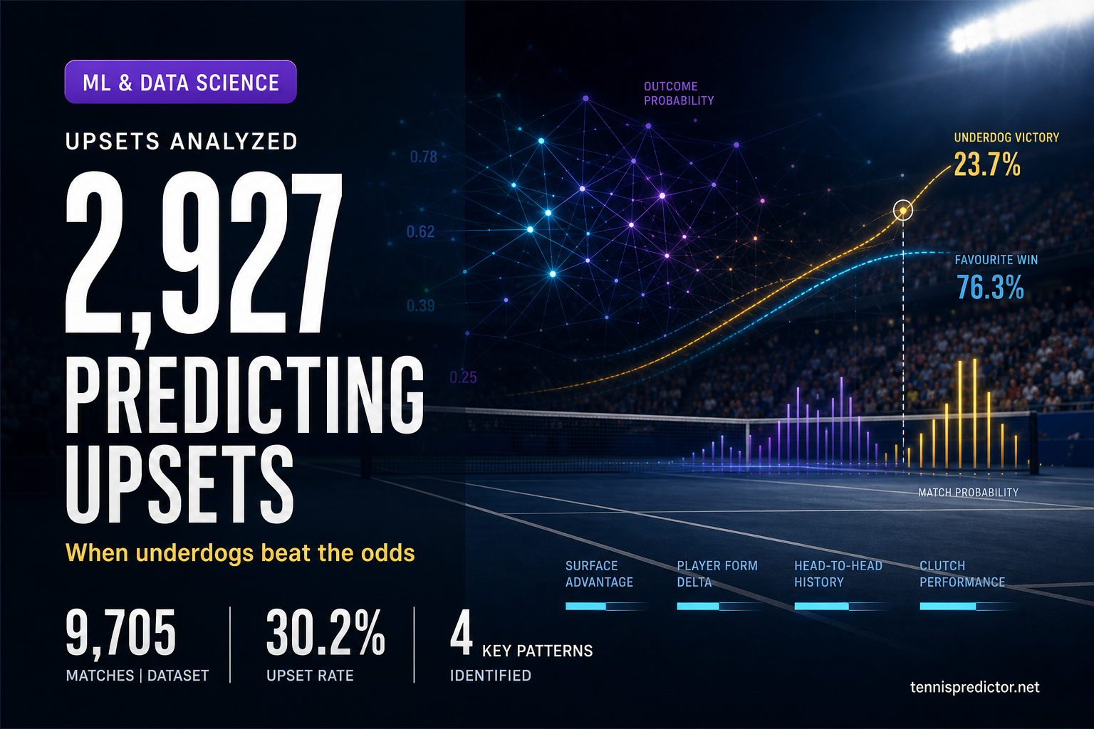
Predicting upsets: how our algorithm spots underdog opportunities
30.2% of tennis matches end in upsets—but they're not random. After analyzing 2,927 upset victories, we've identified four key triggers that appear in 61.8% of underdog wins. Form advantage dominates, rest matters more than you think, and betting markets consistently misprice the 51-100 ranking gap. This is where the value lives.

When our ML model gets it wrong: lessons from failed predictions
October 28, 2025: We predicted Etcheverry to beat Carabelli with 88.4% ensemble confidence. He lost in straight sets. This is the complete failure analysis—the data scarcity (7 indoor matches), the overlooked energy gap, and the five red flags we missed. Transparency matters. Failures teach more than wins.