We analyzed 10,000 tennis matches: here's what we learned
What we mean by “10,000 matches”
The headline rounds up for readability. The exact count in the latest enhanced training export is 9,829 rows—each row is a labelled ATP matchup used in supervised training (winner / loser encoded as the model label). We keep four full seasons in view (2022–2025); the 2025 slice grows as new results are ingested.
Why not import decades of tennis history? Not because “old tennis is useless,” but because our feature pipeline (surfaces, odds coverage, player IDs) is calibrated for the modern tour data we ingest reliably. Expanding backwards is a project, not a spreadsheet toggle.
Matches by year
| Year | Training rows |
|---|---|
| 2022 | 2,647 |
| 2023 | 2,220 |
| 2024 | 2,300 |
| 2025 | 2,662 |
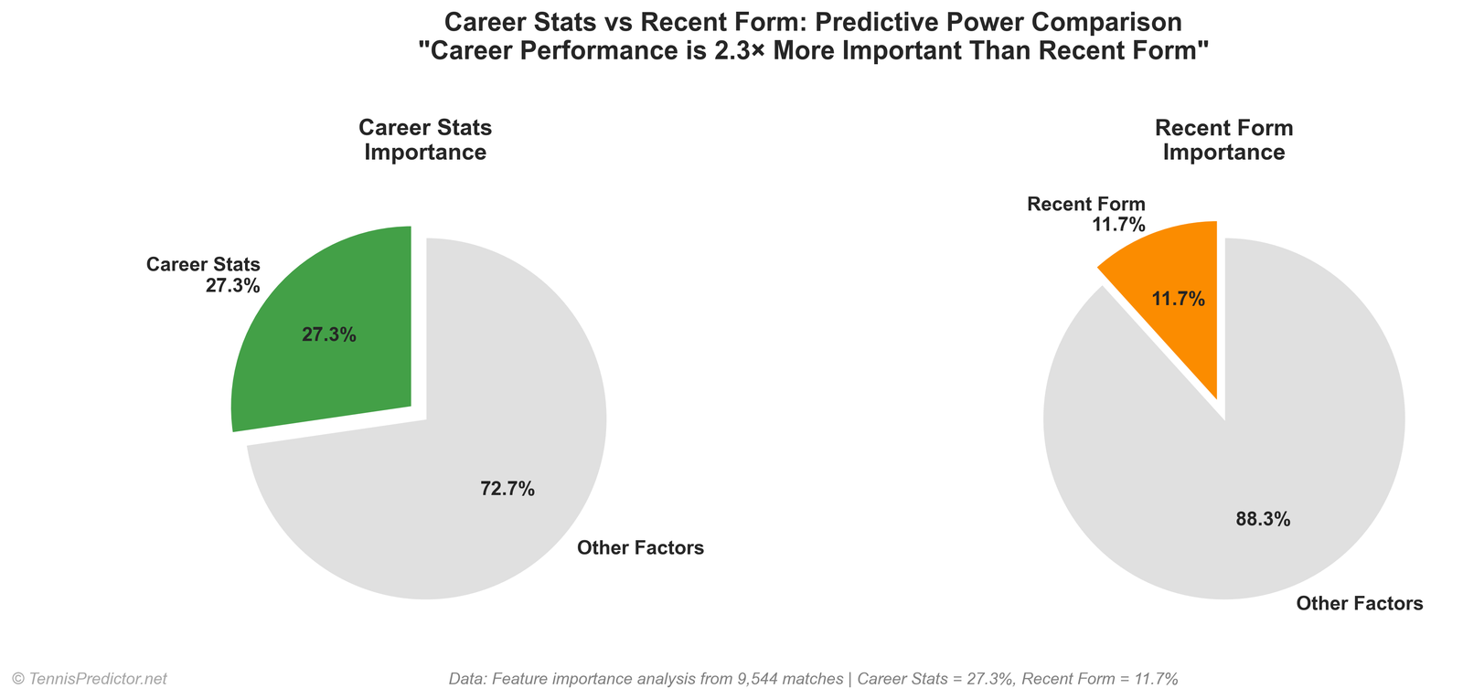
Figure 1: how many labelled ATP matches enter the training file per calendar year.
How to read “feature importance”
We export permutation-style importance shares from the trained Random Forest. Across all features, the shares sum to 100%. That does not mean “the model is 27% odds and 73% heart”—it means: when you ask the forest which inputs it leaned on across trees, a large fraction of the measured signal sits in odds-linked columns.
Grouped sums (importance %):
| Group | Share (sum of importances) |
|---|---|
| Market / odds (implied probabilities, decimal odds, favourite flag, overround, etc.) | 27.38% |
| Player strength (ranks, win rates, experience, interactions) | 28.96% |
| Surface | 16.45% |
| Form / momentum / first-set helpers | 8.60% |
| Other engineered features | 18.11% |
| Head-to-head | 0.50% |
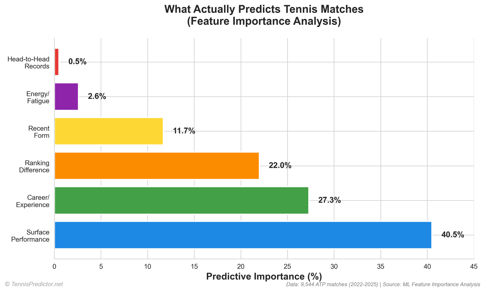
Figure 2: aggregated Random Forest importance by interpretable group.
Plain-language takeaway:
- Books are informative. Odds and implied probabilities aggregate public information faster than any single stat column.
- Player strength still matters—ranks and win-rate differentials are not decorative.
- Surface is material—just not the cartoon version where “clay %” alone explains everything.
- H2H is thin in the aggregate importance table—not because rivalries are meaningless to humans, but because sparse H2H columns rarely beat richer signals at scale.
The top of the leaderboard (exact export)
These are the twelve largest single-feature shares from the Random Forest importance export:
| Rank | Feature (as logged) | Share |
|---|---|---|
| 1 | player2_implied_prob | 6.47% |
| 2 | player1_implied_prob | 5.48% |
| 3 | player1_odds | 4.68% |
| 4 | player2_odds | 4.23% |
| 5 | market_favorite | 2.90% |
| 6 | rank_difference | 2.83% |
| 7 | win_rate_diff | 1.77% |
| 8 | interaction_rank_consistency_p2 | 1.34% |
| 9 | experience_advantage | 1.32% |
| 10 | player1_rank | 1.31% |
| 11 | player2_rank | 1.21% |
| 12 | odds_difference | 1.20% |
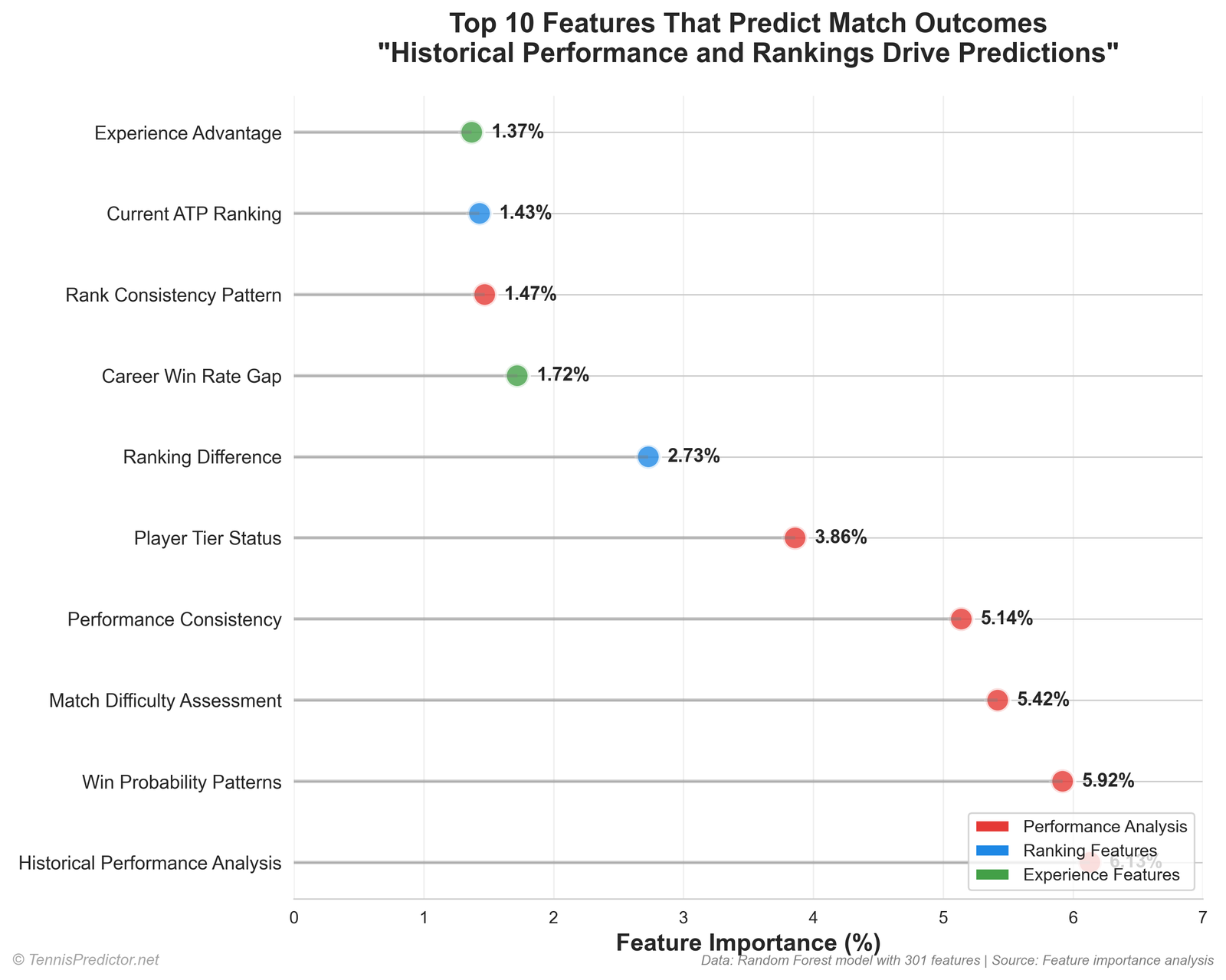
Figure 3: top features by importance share (same export as the table).
If you are betting: treat this as a warning against pure “I ignore the price and only look at form” workflows. The model does not ignore the price—and neither do serious markets.
“Discovery” one — surface matters, in context
You will still see surface performance and surface specialization features in the mid-tier of importance. That aligns with tennis reality: clay reward structures differ from indoor hard courts. What does not align with an older draft of this article is the claim that surface features alone account for 40% of importance. In the current export, the surface bucket is about 16–17% summed—large, but not the whole story.
Practical implication: a clay specialist against a generic hard-court player on clay is still a matchup problem; you should not expect rank alone to do all the work. But you should also not pretend odds are irrelevant just because you watched ten minutes of practice footage.
“Discovery” two — career signal vs last-week stories
Recent form features (rolling win-rate windows and related deltas) appear in the form/momentum bucket (~8.6% combined with first-set helpers). Career-shaped signals (win rates, experience, ranks) sit mostly in player strength. The honest story is not “career is 27% and form is 12%” as literal isolated buckets—those percentages came from an older internal slide deck. The grouped view above is what we stand behind today.
Betting angle: short windows move fast; long windows move slow. Models that only chase the last five scores can overfit noise; models that ignore recent injury or schedule compression can look “smart” on paper and lose in deployment. Our production stack uses both, with the importance table showing you which columns actually carried weight in the latest forest.
“Discovery” three — head-to-head is rarely carrying the forest
Summing every head-to-head feature column yields about 0.5% of total importance. That does not mean “never watch H2H.” It means: in this model, on this feature set, H2H columns are not doing the heavy lifting compared to odds, ranks, and win-rate structure.
When H2H still matters to you as a bettor:
- Large sample on same surface
- Recent meetings (body type, tactics, confidence)
- stylistic mismatches the model may encode elsewhere (serve patterns, lefty spins)
Use video and tactics as overlays, not as a replacement for price discipline.
Underdog wins — define your words
We report rank-based underdog performance: the lower-ranked player (higher ATP rank number) wins the match.
Overall: about 34.51% of training rows are “underdog wins” by that definition.
That is not the same as “the betting favourite lost” (closing-line favourite is a different label). Always check which definition a blog uses before comparing percentages to Twitter threads.
| Tournament level (encoded) | Rows | Underdog win % | Higher-ranked player wins % |
|---|---|---|---|
| Grand Slam | 1,964 | 29.28% | 70.72% |
| Masters 1000 | 2,506 | 35.08% | 64.92% |
| ATP 500 | 1,551 | 33.20% | 66.80% |
| ATP 250 | 3,808 | 37.37% | 62.63% |
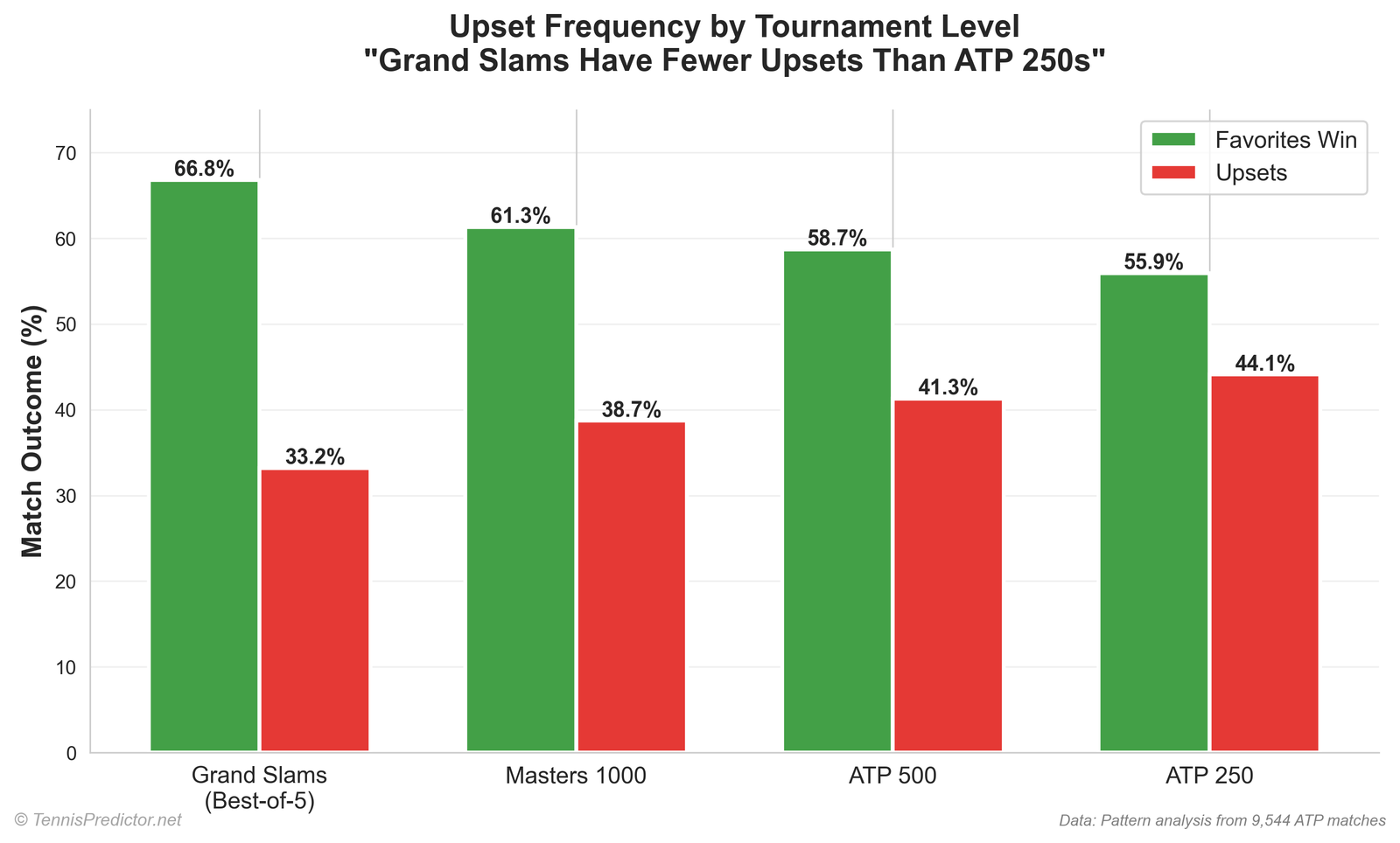
Figure 4: rank-based underdog win share by tournament tier in the training file.
Grand Slam rows show the lowest underdog-win share in this table—consistent with deeper fields and best-of-five for men’s majors (where applicable in the row set).
Ranking gaps — higher-ranked player win rates
Using absolute rank gap buckets (difference in rank numbers between players):
| Abs. gap | Rows | Higher-ranked player wins |
|---|---|---|
| 1–10 | 1,949 | 67.68% |
| 11–20 | 1,213 | 58.70% |
| 21–50 | 3,105 | 63.03% |
| 51–100 | 2,312 | 67.56% |
| 100+ | 1,250 | 70.96% |
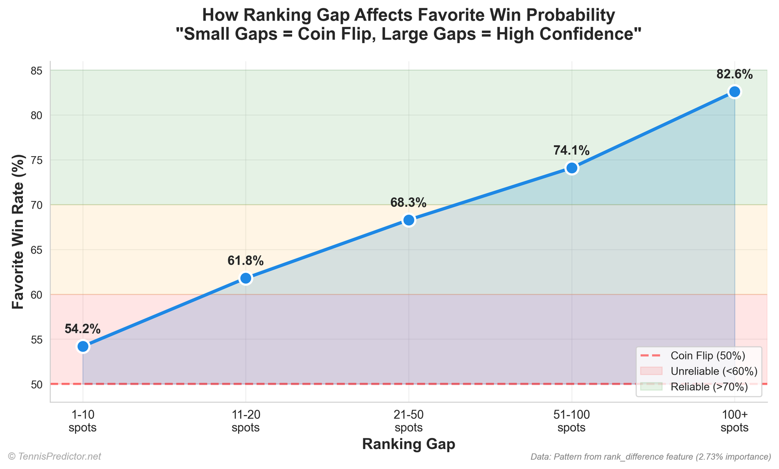
Figure 5: share of matches where the better-ranked player (lower ATP number) wins.
Why the middle bucket looks odd: small gaps are often elite vs elite (tight matches). Huge gaps are often qualifier vs top-five (compressed outcomes). The “21–50” band mixes many different matchup types—always read bucket tables with the sample composition in mind.
First set → match winner
Outcome frequencies for “set one winner also wins match” come from our tournament cache parser (2022–2025), documented in depth in First set wins: the most undervalued betting market?. Headline figure: 69.1% over 9,698 parseable matches.
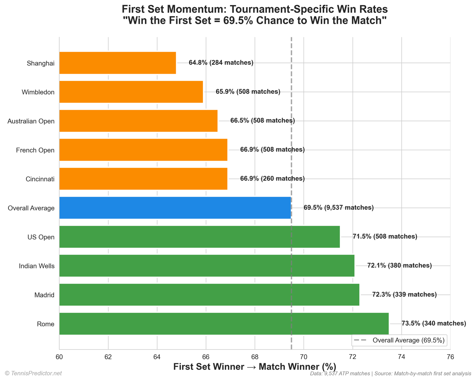
Figure 6: overall first-set winner match-win share (cache aggregate).
Do not confuse that number with fair odds for betting set one—it is a historical joint frequency, not a price.
Odds vs “pure stats”: a tension every serious model faces
New readers sometimes bristle when they see implied probability near the top of an importance table. The discomfort is understandable: it can feel like the model is “cheating” by peeking at the price.
Here is the cleaner mental model:
- Odds are inputs, not labels. The label is still who won. The forest learns residual structure—places where player history, surface splits, and schedule features push outcomes away from what a naive market-implied probability might suggest, when those deviations are stable enough to generalise.
- Markets can be sharp and still leave structure. Tennis has thin samples, late withdrawals, and stylistic mismatches. A model’s job is not to prove the market stupid every Tuesday; it is to combine public prices with structured history under honest testing.
- If your fair probability matches the implied price, you may have no edge—even if the model’s headline accuracy sounds impressive. Edge is price-relative in betting, not vibes-relative.
That framing is why we publish multiple evaluation views (cross-validation, holdout, live KPI) instead of a single heroic percentage. A single number rarely survives contact with deployment.
Correlation, importance, and what forests cannot prove
Random Forest importance tells you which inputs co-occurred with better splits in training data. It does not automatically prove causality:
- Collinearity: rank, win rate, and odds often move together for the same player. Importance shares can shift when you retrain on a new season mix.
- Leakage vigilance: we use chronological protocols for evaluation so we do not “peek” at the future when measuring generalisation. Importance on the training object is still not a substitute for a clean forward test.
- Calibration: a model can be directionally useful while still needing probability calibration work—especially at the tails (heavy favourites).
If you want a philosophical companion piece on engines and baselines, read Machine learning vs statistical models: which predicts tennis better?.
Model accuracy: three numbers, three questions
This article is not the place to claim a single “83.8% model accuracy” headline. Read How our AI predicts tennis matches with 70%+ accuracy for:
- Cross-validation (~79.5% in the latest export)
- Chronological holdout (~63.1%)
- Live settled hit rates (rolling samples; smaller n)
Those three answers coexist because they measure different things. Mixing them is how social media gets loud and wrong.
A practical workflow for readers who bet (without cosplaying as a quant)
You do not need to read a 300-feature schema to apply one disciplined workflow:
- Write down a fair win probability — from a model, from your own research, or from an average of both.
- Convert the posted odds to implied probability (remember margin).
- Ask whether the gap survives vig and whether your sample size for the specific player context is large enough to trust.
- Size stakes to uncertainty — wide bands should mean smaller stakes, even when the “pick” is the same.
This is the same “probability first, story second” discipline we try to apply internally when discussing value versus accuracy. For a beginner-friendly tour of value thinking, see Value betting in tennis: a beginner's guide.
Sampling notes: why gaps and upsets are easy to misread
Two traps show up constantly in tennis analytics threads:
Trap A — treating one bucket table as destiny.
A bucket like “21–50 rank gap” mixes wildly different match types: some are two top-20 players separated by thirty ranking places because one missed time; others are #5 vs #60 in early rounds. The bucket average is a marginal distribution, not a forecast for your specific card.
Trap B — confusing “underdog by rank” with “plus-money by closing line.”
Closing lines incorporate injuries, rumours, and liquidity. Rank gaps do not. Our upset tables are descriptive slices of the training file, not a claim that sportsbooks misprice every underdog.
If you want a tournament-level lens on predictability that uses different cuts, pair this article with The Grand Slam betting guide: majors vs ATP 250s—not because it repeats the same numbers, but because it reinforces the idea that format and field change risk.
What we fixed in this 2026 rewrite
Earlier versions of this page mixed aspirational importance percentages, stale match counts, and illustrative chart scripts. This revision ties prose to:
- 9,829 training rows in the current export
- The Random Forest importance export for tables and figures
- Rank-based underdog and gap statistics from the same pipeline
- First-set headline aligned with the refreshed first-set article
If a future training export changes the top feature order, refresh the importance export and re-run the extraction script—do not hand-edit percentages to match a narrative.
Limitations
- ATP training rows only here—WTA and challengers are different coverage stories.
- Importance ≠ causal effect—permutation importance can shift when features correlate.
- Rank-based underdog is not the same as closing-line upset.
- Odds features encode market wisdom; beating the line still requires edge vs price, not edge vs your memory.
- Feature lists evolve as we add columns and retrain; always trust the current importance export for the live model, not a screenshot from an old blog revision.
- Class balance and tournament mix in the training file influence what the forest can learn—aggregates are stable enough for education, but not a substitute for a full modelling review.
Glossary (quick)
- Implied probability: win chance embedded in decimal odds before adjusting for book margin (roughly (1 / \text{odds}) per side in a simple two-way market).
- Permutation importance: a way to score how much model accuracy suffers when a feature’s values are shuffled—here reported as share summing to 100% across features.
- Higher-ranked player: the player with the lower ATP rank number (better ranking).
- Underdog (rank-based): the player with the higher ATP rank number (worse ranking).
Responsible betting
Use bankroll limits. Treat any percentage as historical context, not a promise. If betting stops being fun, seek help early.
Frequently asked questions
1. Is it exactly 10,000 matches?
No. The current file has 9,829 training rows; we round in the title for scanability and explain the exact count up front.
2. Why do odds features rank so high?
Bookmakers aggregate public and private information quickly. Odds-derived columns act as a compressed consensus sensor—the model still blends them with player and surface history.
3. Is surface irrelevant?
No. The surface bucket is roughly one-sixth of summed importance in the latest export—far from irrelevant.
4. Should I ignore head-to-head completely?
Not as a human. Statistically, H2H columns are thin versus other signals in this forest—but repeated stylistic matchups can still matter to your process.
5. What is an “upset” in your tables?
Here, lower-ranked player wins (higher ATP rank number). That is not identical to “favourite lost at closing odds.”
6. Why do Grand Slams show fewer rank-upsets than ATP 250s?
Partly field strength, partly format, partly who enters the draw—interpret with care.
7. How often does the first-set winner take the match?
About 69.1% in our 2022–2025 ATP cache parse—see the first-set article for methodology.
8. What accuracy should I believe?
Read the AI article: CV, holdout, and live answer different deployment questions.
9. Can I reproduce these tables?
Yes—re-run the extraction script bundled with this article’s generator assets (outputs JSON alongside the markdown).
10. Where do I see live predictions?
Open the predictions dashboard.
11. Does this article replace feature engineering docs?
No. For intuitive feature descriptions, see The secret sauce: features that power our tennis predictions.
12. What should I read next for market mechanics?
Best tennis markets to bet: match winner vs set betting vs games.
13. Why did an older version of this article quote different percentages?
Training data grows, features change, and bad charts happen when marketing copy outruns the export pipeline. This 2026 revision is pinned to the current CSVs named in the transparency section.
14. Do you publish the raw training file?
We publish aggregates and methodology; the full training matrix is large and tied to internal pipelines. The important part for readers is that the blog numbers are reproducible from named exports, not hand-tuned.
15. Can surface still be “the decider” in an individual match?
Yes—especially when one player is a structural specialist and the other is not. The importance table says surface is not the only decider at the model level, not that surface is irrelevant on court.
16. How do I interpret “importance” without overfitting myself?
Feature importance is a post-hoc summary of what the forest leaned on after training. It is not a causal statement (“surface causes wins”) and it is not a guarantee that removing a group would drop accuracy by exactly that percentage. Treat it as:
- A ranking hint for which signals are informative in aggregate.
- A sanity check against marketing claims (“H2H decides everything”).
- A starting point for ablation studies and error analysis.
If two groups overlap in meaning (market-implied strength versus rank-based strength), do not sum their shares as if they were independent causal levers. Use the table as a map, not as a precise ledger.
17. What are the main limitations of this analysis?
- Historical slice: Patterns describe the training window in the CSV, not a universal law of tennis.
- Label definition: The model predicts match outcomes from pre-match features; it does not model rally-by-rally dynamics beyond what the columns encode.
- Importance method: Random Forest importance can be biased toward high-cardinality or continuous features; grouped buckets reduce but do not remove that bias.
- Tournament tables: Small-sample events can look extreme; use them as context, not as stable rules you can quote forever.
Related reading
- How our AI predicts tennis matches with 70%+ accuracy
- Machine learning vs statistical models: which predicts tennis better?
- First set wins: the most undervalued betting market?
- The decisive set: third set & fifth set statistics that matter for bettors
How this piece fits next to the “features” article
The secret sauce: features that power our tennis predictions explains what we measure in plain language—surface splits, form windows, energy, and more. This article answers a different question: which buckets dominate the latest Random Forest importance export, and how to interpret those shares without overdramatising any single column.
If the two pages ever feel like they “disagree,” check the date and the export:
- Feature article prioritises intuition and coaching-style explanations.
- This article prioritises auditability against the current importance export.
Both can be true: a feature can be conceptually important to humans while sharing importance mass with correlated columns inside a tree ensemble.
Rows, columns, and the illusion of “one true model”
The training matrix currently ships roughly 300 numeric columns before labels and IDs—not all of them are independent. Trees thrive on interactions; that is why you see rank–consistency interaction terms mid-table: they capture non-linear combinations that linear dashboards would hide.
None of that means the model is omniscient. It means: if you try to reduce tennis to one stat, you will be surprised by trees that keep using odds and rank gaps anyway, because those columns stabilise decisions on messy weeks.
Correlation reality check: many features move together—better players post better win rates, attract shorter prices, and accumulate ranking points. Importance splits those joint movements across correlated columns. That is another reason grouped buckets are useful: they stop you from triple-counting the same underlying “who is better?” signal under three different names.
Data transparency
Aggregates in this article were generated from:
- The latest enhanced training export (row counts, rank-gap tables, tournament-level upset rates).
- The feature importance export from the trained Random Forest (top features and grouped sums).
- First-set headline figures for Figure 6 from the same cache pipeline as First set wins: the most undervalued betting market?.
After each major training refresh, re-run:
cd website_generator
python3 extract_article_04_training_stats.py
python3 create_article_04_charts.py
That keeps figures, tables, and prose aligned without hand-editing percentages.
Closing
Big-sample tennis writing should feel boring in the right ways: explicit definitions, reproducible tables, and no fairy tales about secret 80% accuracy shortcuts. The data we actually train on says markets and player-strength signals dominate the importance ledger, surface still matters, H2H features are thin in aggregate, and rank-based underdogs still win often enough that risk management always comes first.
For prices you can bet today, start at the dashboard—after you have read what the numbers mean.
See today's match predictions with confidence scores and value signals.
View Live Predictionsarrow_forwardRelated Articles
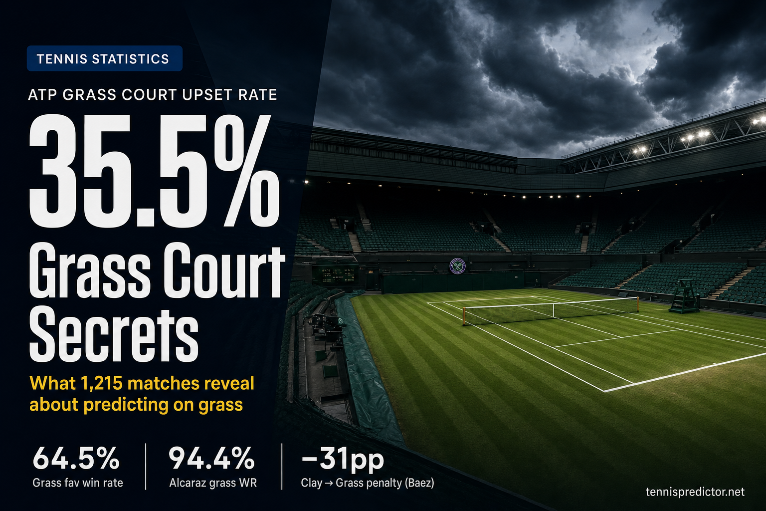
ATP grass court specificity: what 1,215 matches really tell us
Everyone repeats the same myths about grass — that it's random, that serve specialists always win, that clay court form means nothing. Our model disagrees. We dug into 1,215 ATP grass matches from 2022 to 2025 to separate the folklore from the numbers.
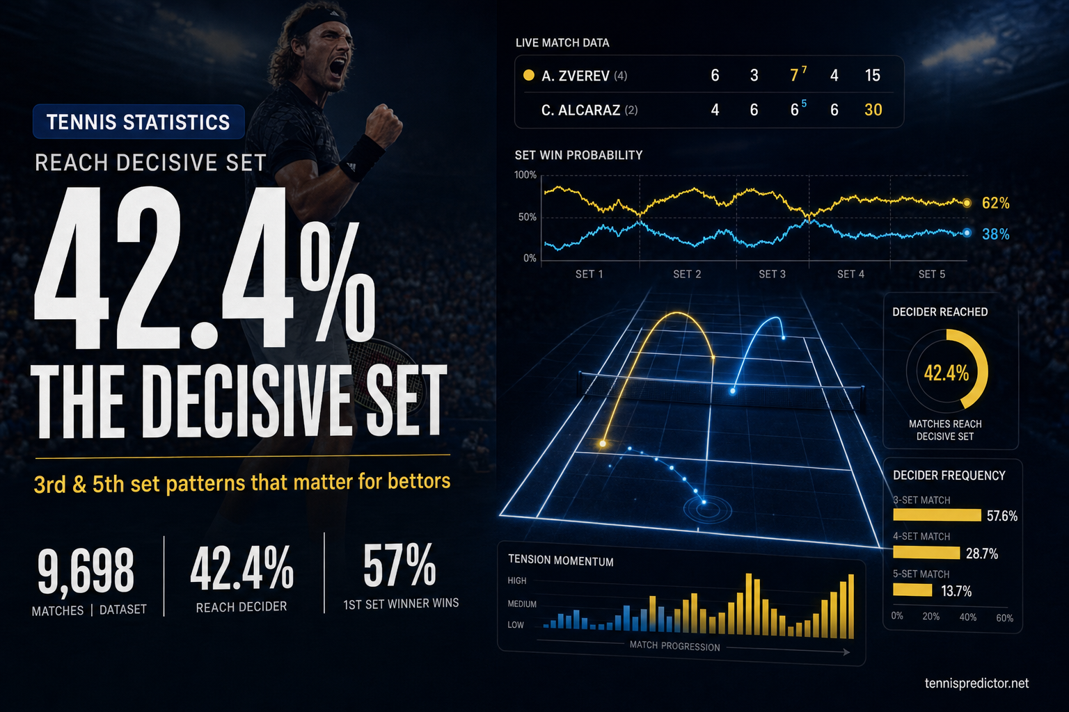
The decisive set: third set & fifth set statistics that matter for bettors
How often do ATP matches go to a third or fifth set—and when they do, does the first-set winner usually close it? Real scorelines, Grand Slam vs tour splits, and what it means for set and live betting.
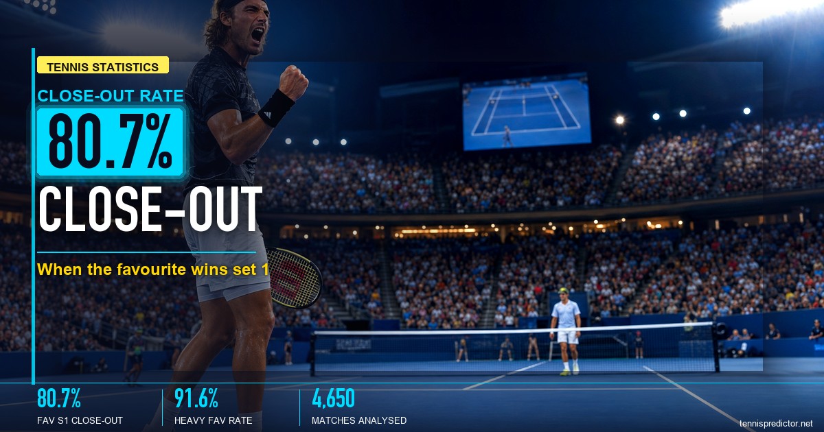
When the favorite wins the first set: match close-out rates by surface and odds
When a pre-match favourite wins the first set, they close out the match 80.7% of the time — a 12-point boost over their baseline. But that number swings from 66% to 94% depending on their odds and the surface. Here's the full data-backed breakdown across 4,650 ATP matches.
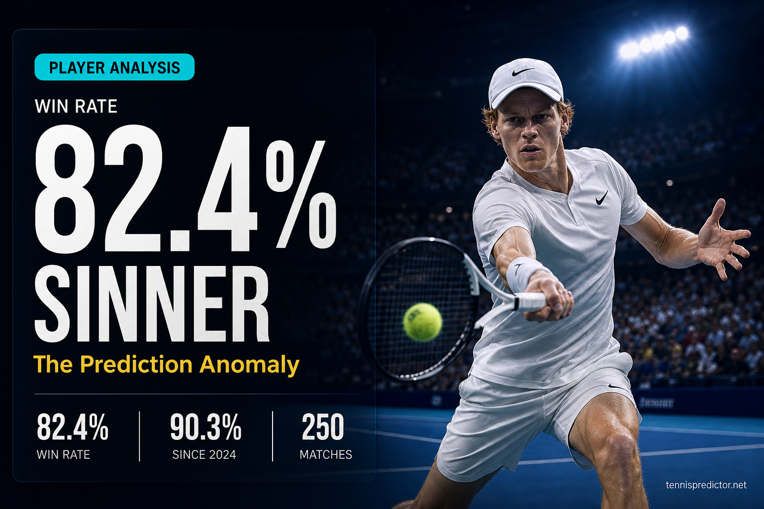
Jannik Sinner: the rise of a prediction anomaly
Sinner won 249 matches at 82.3% between 2022 and 2025 — and that number has only trended upward. We analysed every surface, round, and elite matchup to explain the prediction paradox: he is simultaneously the easiest player to predict and the hardest to beat.