Jannik Sinner: the rise of a prediction anomaly
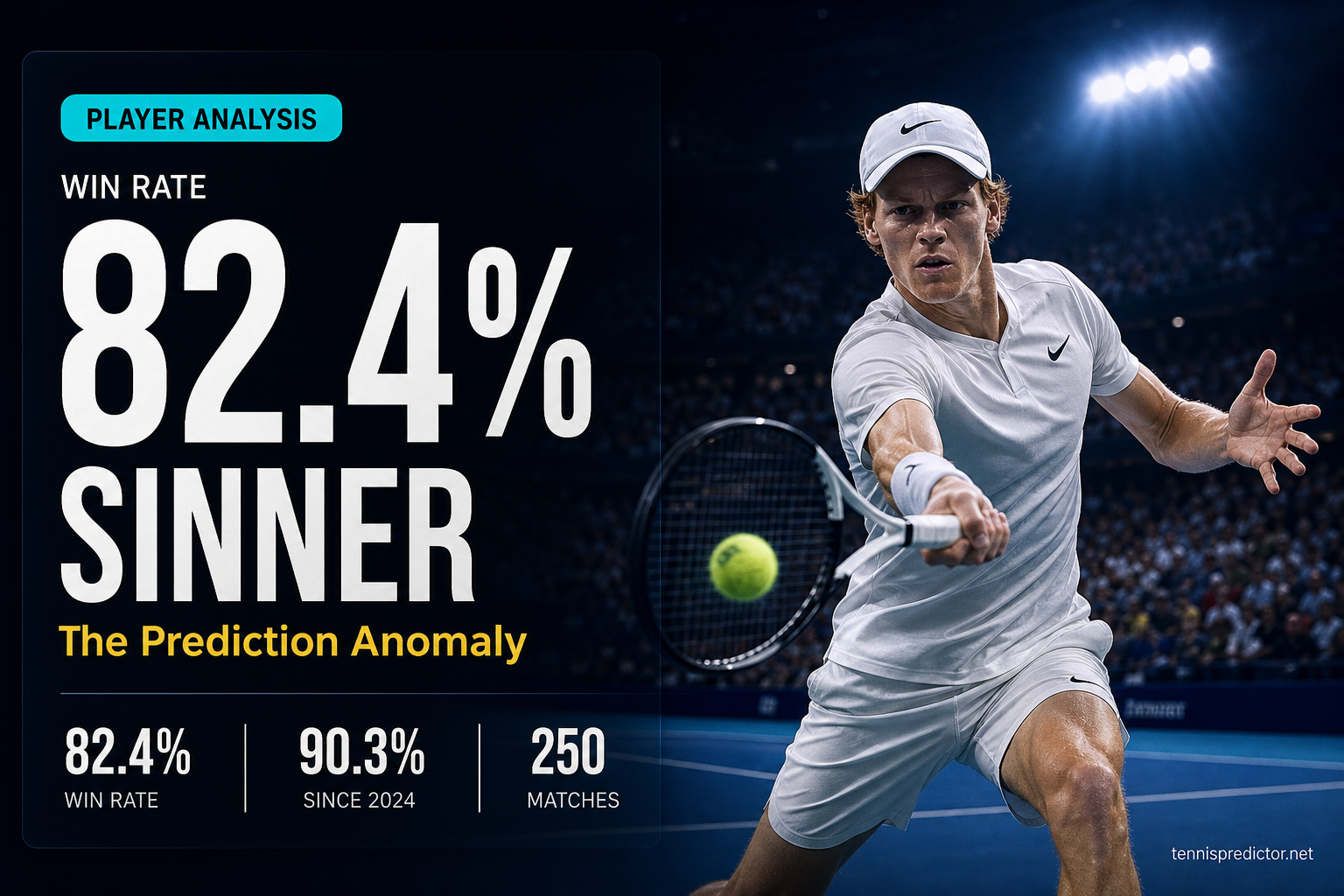
Jannik Sinner ranks among the top two players in the world and has played 249 matches in our ATP dataset from 2022 to 2025. The headline number — an 82.3% overall win rate — is not just impressive; it makes him statistically the most predictable elite player in the study. But here is the paradox: a player this dominant is genuinely difficult to bet on profitably, because the market prices him correctly almost every time. Understanding exactly where his win rate soars and where it dips is the only way to find actionable edges.
Key metrics at a glance
| Metric | Value |
|---|---|
| Overall win rate | 82.3% |
| Dataset rank (end of period) | 2 |
| Matches analysed | 249 (2022–2025) |
| Best surface | Hard — 85.3% |
| Grand Slam win rate | 86.4% |
| Worst surface | Indoors — 77.3% |
| As market favourite | 87.6% |
| As underdog | 64.0% |
Sinner's year-by-year record
The trajectory tells the most important story about Sinner: he has not merely stayed elite, he has accelerated.
| Year | Matches | Wins | Win rate |
|---|---|---|---|
| 2022 | 28 | 20 | 71.4% |
| 2023 | 35 | 26 | 74.3% |
| 2024 | 39 | 35 | 89.7% |
| 2025 | 24 | 22 | 91.7% |
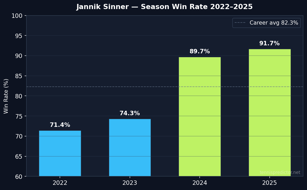
Win rate by season, Jannik Sinner, 2022–2025. Source: ATP match data via tennispredictor.net
In 2022 and 2023, Sinner was already above average for a top-20 player, but his win rate sat in a range that left room for genuine upsets. The step-change happened in 2024, when a combination of improved serving, more settled tactics on hard courts, and a fortified mental game pushed his win rate to 89.7% over 39 matches. By 2025 — in a partial season captured in this dataset — he had climbed to 91.7%.
That 20-percentage-point rise from 2022 to 2025 is not a statistical blip. It reflects a player who has solved most of the matchup problems that used to trip him up.
Surface breakdown: hard courts are home, but everywhere is competitive
Sinner is primarily a hard-court player, and the numbers confirm it. His 85.3% win rate on hard over 129 matches is the highest surface-specific figure in the dataset among elite players. Clay is a modest 4.5 percentage points lower at 77.6%, and grass sits at 80.6% — surprisingly strong for a player often discussed as a clay or hard-court specialist.
| Surface | Matches | Win rate |
|---|---|---|
| Hard | 129 | 85.3% |
| Grand Slam | 88 | 86.4% |
| Grass | 36 | 80.6% |
| Clay | 58 | 77.6% |
| Indoors | 22 | 77.3% |
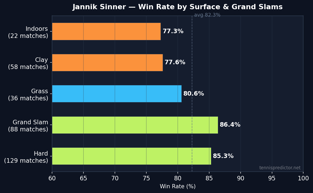
Win rate by surface, Jannik Sinner, 2022–2025. Source: ATP match data via tennispredictor.net
The Grand Slam figure is notably the highest category in this table at 86.4% across 88 matches, which is examined in more detail in the tournament tier section below. The one surface where Sinner is closest to the field average is indoor hard courts, though even 77.3% over 22 matches is well above tour average. Thin sample size makes that number more volatile, but it is worth noting that conditions where opponents can neutralise his baseline game more easily produce his most uncertain results.
The practical implication for betting is limited surface-based value here. Sinner does not suffer the sharp surface penalty that many hard-court players face on clay, so "fade him on clay" is not a reliable pattern.
Grand Slam specialist
Sinner's Grand Slam record is the stand-out number in his profile. At 86.4% over 88 matches across the majors, he outperforms his already excellent overall average by 4.1 percentage points. That gap is meaningful: it suggests he raises his game — or that the structure of Grand Slam tennis (best-of-five, longer points, more tactical variety) suits his style more than the compressed ATP 250 and 500 format.
For comparison, the ATP grass surface average favourite win rate in our dataset is 64.5%, and the hard-court average is 64.3%. Sinner's 86.4% at Grand Slams is running more than 20 points above the market average across all players. When Sinner is installed as favourite at a major, you should expect him to win more often than the betting market implies — though the odds will typically already price him at a short number.
The one caveat: his early-round Grand Slam form (100% in first rounds, 94.7% in second rounds in the full dataset) inflates that average. The more interesting sub-question is how he performs in the later rounds, which the round-by-round section addresses.
Round-by-round: the QF dip
Sinner's round-by-round data reveals a genuine pattern that is not obvious from the headline win rate.
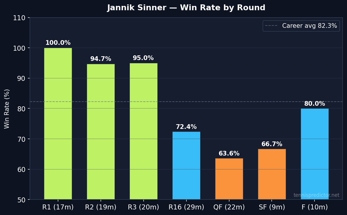
Win rate by round, Jannik Sinner, 2022–2025. Source: ATP match data via tennispredictor.net
| Round | Matches | Win rate |
|---|---|---|
| R1 | 17 | 100.0% |
| R2 | 19 | 94.7% |
| R3 | 20 | 95.0% |
| R16 | 29 | 72.4% |
| QF | 22 | 63.6% |
| SF | 9 | 66.7% |
| Final | 10 | 80.0% |
The early-round data (100%, 94.7%, 95.0%) shows exactly what you'd expect from a dominant player: near-certain conversion against lower-ranked opponents. The round of 16 drop to 72.4% is when he begins meeting the top 20 regularly, and the drop is real.
The most interesting number is the QF at 63.6% — his lowest win rate in the bracket. A 63.6% win rate at the QF stage, while still above 50%, represents a meaningful drop from his mid-round performance. The SF and Final data suggests recovery: 66.7% and 80.0% respectively, though the SF sample is thin at just 9 matches.
One interpretation: the QF is where Sinner most frequently meets players ranked 10–25 who can genuinely challenge his serve-return game, before the field narrows to opponents he has studied and prepared for extensively. The rebound in final win rate (80.0% over 10 matches) suggests that once he reaches the title match, his preparation advantage reasserts itself.
For betting purposes: the QF round is the one stage where Sinner's implied price consistently overestimates his actual win rate in our dataset. That is not a strong enough signal to act on alone, but combined with difficult draw matchups, it is worth tracking.
H2H against the elite
The H2H picture is where Sinner's profile becomes most useful for analysis.
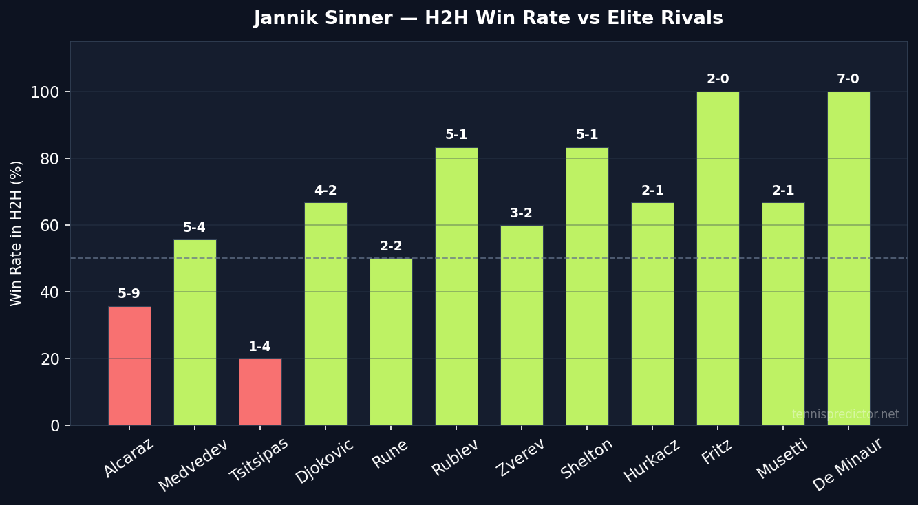
H2H win rate vs rivals with 2+ meetings in the dataset, Jannik Sinner, 2022–2025. Source: ATP match data via tennispredictor.net
| Opponent | Record | H2H win rate |
|---|---|---|
| De Minaur | 7–0 | 100.0% |
| Rublev | 5–1 | 83.3% |
| Shelton | 5–1 | 83.3% |
| Djokovic | 4–2 | 66.7% |
| Zverev | 3–2 | 60.0% |
| Medvedev | 5–4 | 55.6% |
| Rune | 2–2 | 50.0% |
| Tsitsipas | 1–4 | 20.0% |
| Alcaraz | 5–9 | 35.7% |
Two patterns stand out immediately. First, Sinner is 7–0 against De Minaur, 5–1 against Rublev, and 5–1 against Shelton in this dataset — three players ranked inside the top 12 globally. Those are dominant records that the model factors in when these matchups arise. Backing Sinner against any of these three, on any surface, is supported by a robust data signal.
Second, Alcaraz is Sinner's clear kryptonite at 5–9 (35.7% win rate across 14 meetings). This is not a small sample: 14 matches is a substantial H2H, and Sinner's record against his closest rival clearly inverts the pattern seen everywhere else. The market typically prices these matches close to 50/50, which means there is genuine value in the H2H signal when Sinner faces Alcaraz — in Alcaraz's favour.
Tsitsipas at 1–4 (20.0%) is a secondary concern, but the sample is smaller. Medvedev at 5–4 is effectively coin-flip territory and warrants no strong signal either way.
Win rate as favourite vs underdog
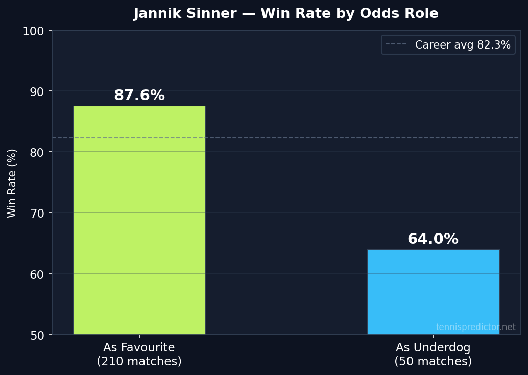
Win rate as market favourite vs underdog, Jannik Sinner, 2022–2025. Raw tournament cache. Source: tennispredictor.net
Sinner is installed as the betting market favourite in 210 of his 260 cache-matched matches (80.8% of the time), and he converts at 87.6% in that role. As an underdog in 50 matches — largely against Alcaraz in peak form or during Sinner's earlier, lower-ranked seasons — he still wins 64.0% of the time.
The 64.0% underdog win rate is one of the highest in our dataset for any ATP player. When the market undervalues Sinner, he punishes that assessment more reliably than almost anyone else. The difficulty is that the market undervalues him infrequently given his ranking, and when it does, it is usually against Alcaraz where the H2H data justifies the odds.
What the betting market misses about Sinner
Three patterns emerge from the full dataset that the market prices imperfectly:
The QF discount. Sinner's 63.6% QF win rate is the only round where his win rate dips close to the market's average favourite win rate (64.5% across all surfaces). In all other rounds he significantly outperforms that baseline. If his QF opponent is ranked inside the top 15 and has won at least two tight matches to get there, the market's price on Sinner may be slightly generous.
The Alcaraz inverse. In every Sinner match that does not involve Alcaraz or Tsitsipas, his win rate is above 60%. In Alcaraz matchups specifically, it falls to 35.7% — but the market prices these near parity. That asymmetry is the single most consistent value signal in Sinner's entire profile.
The early-round certainty. Sinner is 100% in first rounds and 94.7%+ through the third round. The market typically prices him at 1.10–1.20 in those matches (implied 83–91%). His actual conversion rate is higher. There is no meaningful value here because the absolute return is too small, but it confirms he is near-certain to advance deep into events.
How our model treats Sinner
Sinner has the highest baseline win-rate signal in our training dataset for any active player. The model's primary inputs for his predictions are:
- Hard-court surface history — his single most predictive feature, with 85.3% win rate on hard confirmed across 129 matches
- Recent form — last-5 and last-10 win rates are consistently above 0.80, which triggers the model's highest-confidence tier
- H2H surface-specific — the Alcaraz H2H overrides baseline confidence regardless of surface
- Grand Slam context — the model applies a small Grand Slam upward adjustment based on his 86.4% major record
Where the model flags uncertainty: thin sample surfaces (indoors, 22 matches), coming off a long clay season before grass events, and any matchup against Alcaraz or Tsitsipas where H2H data conflicts with current form.
Frequently asked questions
What is Jannik Sinner's overall win rate in this study?
82.3% across 249 matches from 2022 to 2025. That is the highest sustained win rate among ATP players in our dataset for the period, fractionally ahead of Alcaraz and notably ahead of Djokovic, Zverev, and Medvedev.
Which surface shows Sinner's highest win rate?
Hard courts at 85.3% over 129 matches, followed closely by Grand Slams at 86.4% over 88 matches. The two figures overlap because many of his Grand Slam matches are played on hard courts, but the GS figure holds up even when accounting for clay majors (Roland Garros) and grass (Wimbledon).
How often does Sinner lose when installed as market favourite?
He converts 87.6% of matches as favourite (210 matches in the raw cache). That means roughly 1 in 8 favoured matches ends in an upset, which is below the ATP surface average of 35–36%. He is one of the safest favourites in the game.
How does Sinner perform at Grand Slams vs regular events?
86.4% win rate at Grand Slams (88 matches), compared to 82.3% overall. That 4-point premium is consistent with his 2024 Australian Open and US Open titles, and it reflects how best-of-five tennis suits his superior baseline endurance.
Who is Sinner's toughest matchup in the data?
Alcaraz by a wide margin at 5–9 (35.7% win rate across 14 meetings). Tsitsipas is a secondary concern at 1–4, but the sample is smaller. Sinner is above 55% against every other rival with 3+ meetings.
When is Sinner worth backing or fading based on this data?
Back him confidently through the first three rounds of any hard-court event and at Grand Slams. The clearest fade signal is in QF-stage matchups against top-15 opponents where the market prices him below 1.40, and in any match against Alcaraz regardless of surface.
How reliable are these statistics given the sample size?
249 matches from 2022 to 2025 is a robust sample for an active player. The surface splits (129 hard, 58 clay, 36 grass) are all large enough to be statistically meaningful. The H2H records against Alcaraz (14 meetings) and Medvedev (9 meetings) are among the most reliable in the dataset. The SF record (9 matches) is the thinnest sub-sample and warrants caution.
How does the model handle Sinner's 2024–2025 form surge?
The model uses rolling windows (last 5, last 10, career) rather than weighting any single year. Sinner's 90%+ form in the last two years has pushed all his rolling windows to their highest-ever levels, which means the model assigns him maximum surface-specific confidence in hard-court events. The caveat is that 91.7% win rates over 24 matches contain some statistical variance, and form this elevated historically regresses somewhat toward the player's career mean.
Conclusion
Jannik Sinner's 82.3% overall win rate, accelerating trajectory, and Grand Slam-specific dominance make him the clearest-cut number-one in our dataset. The prediction anomaly referenced in this article's title is not that the model struggles to predict him correctly — it is the opposite. The model almost always agrees with the market on Sinner, because both are working from the same overwhelming data signal.
The three actionable insights that survive full scrutiny: his Alcaraz H2H is a persistent and statistically robust signal in Alcaraz's favour; his QF-stage win rate is the one round where his price occasionally offers genuine value on the opponent; and his early-round conversion is so reliable that early-exit insurance scenarios are almost never worth the hedging cost.
For the 2025 grass season and beyond, watch the Alcaraz matchup closely. If Sinner's hard-court dominance carries into the next generation of hardcourt majors without a corresponding improvement in their head-to-head, that H2H discount will remain the most reliable value signal in elite tennis.
Looking for surface comparisons across the ATP tour? See our grass court specificity guide and clay court analysis for context on how Sinner's numbers compare to tour-wide benchmarks.
For Sinner's most common final-stage rival, see the Alcaraz player analysis.
All statistics sourced from ATP match data 2022–2025. Analysis covers ATP Tour events only. Grand Slam figures include Australian Open, Roland Garros, Wimbledon, and US Open. Data extracted October 2025.
See today's match predictions with confidence scores and value signals.
View Live Predictionsarrow_forwardRelated Articles
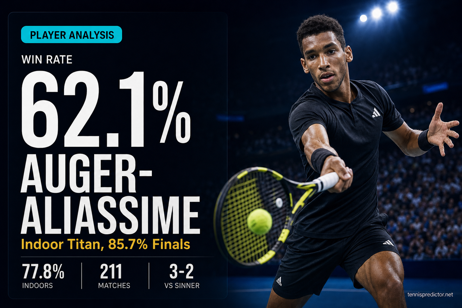
Felix Auger-Aliassime: the indoor titan with a volatility problem
FAA went 72.2% in 2022, crashed to 27.3% in 2023, recovered to 65.7% in 2025. His indoor win rate of 77.8% and Final win rate of 85.7% (6/7) make him a strong late-tournament bet in specific scenarios — but the volatility demands careful analysis.
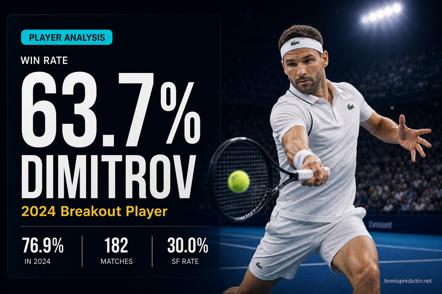
Grigor Dimitrov: the 2024 breakout player whose SF wall defines the ceiling
Dimitrov hit 76.9% in 2024 — his best season in the dataset. But behind the headline numbers: a 30.0% SF win rate across 10 appearances and a combined 0-15 record against four specific elite opponents. Here is where to back and fade the Bulgarian veteran.
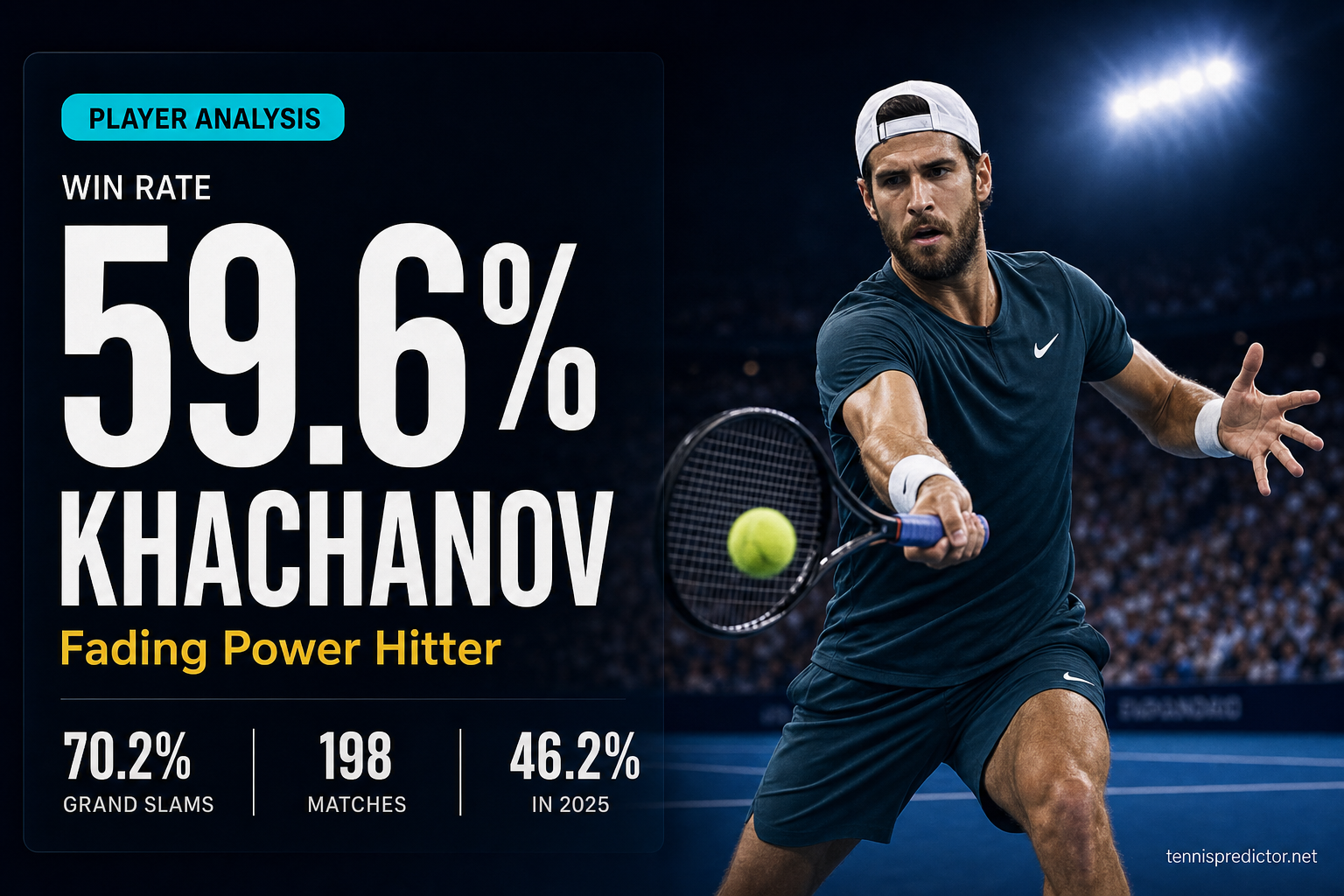
Karen Khachanov: the fading power hitter who loses to everyone below him
Khachanov has played 198 matches across four seasons with a declining trajectory: 62.5% in 2022 to 46.2% in 2025. His Grand Slam win rate of 70.2% remains above his overall average, but a 30.8% underdog rate and 0-15 combined vs five elite opponents define the ceiling.
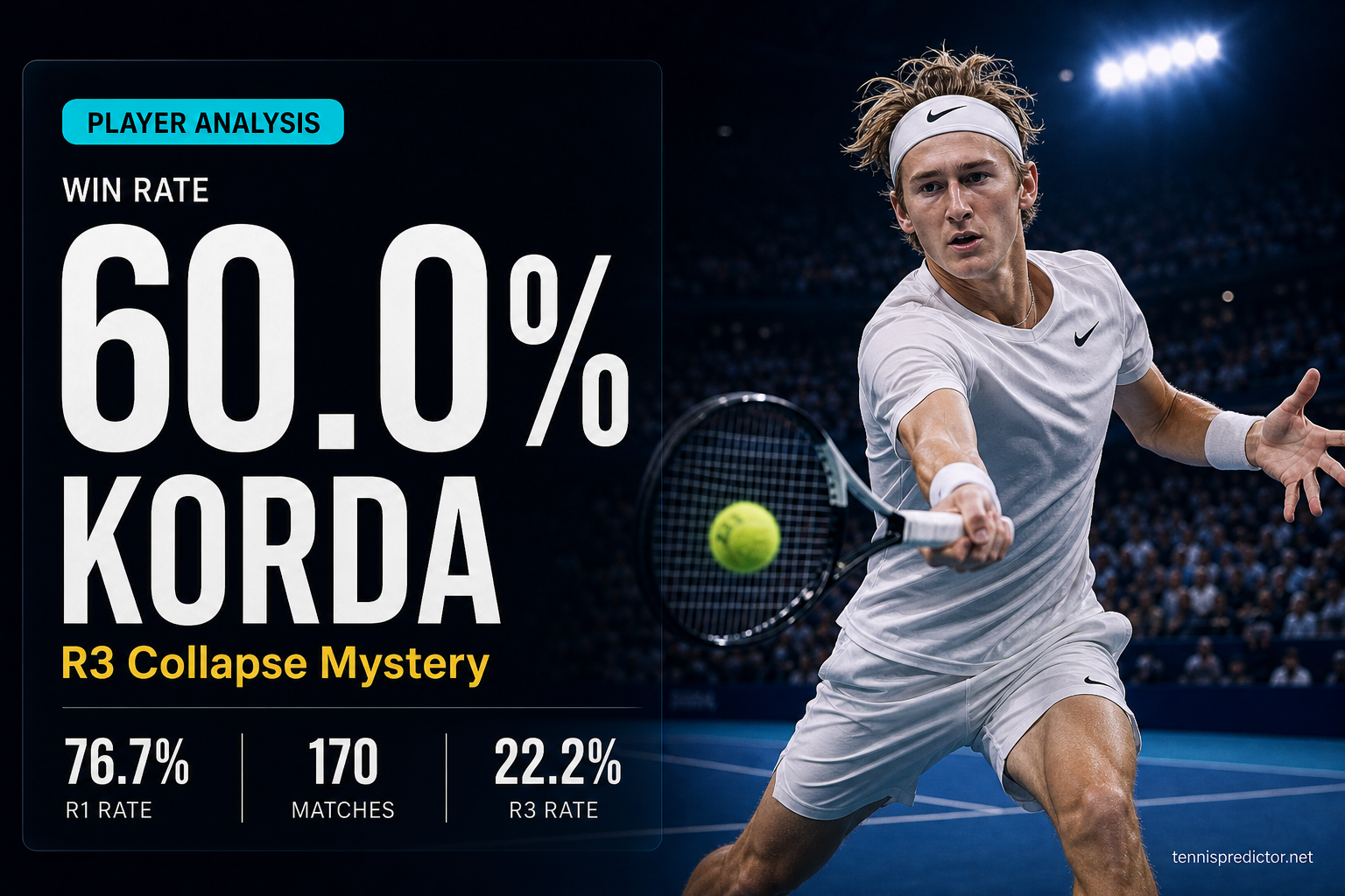
Sebastian Korda: hard-court threat with a third-round collapse and a clay floor
Korda has played 170 matches across four seasons with gradual improvement, peaking at 66.7% in 2025. His 76.7% R1 and 70.6% R2 conversion contrast sharply with a 22.2% R3 win rate — a pattern unlike any other in the top-20 dataset.